


Understanding Resnet
ResNet has been a very influential architectural optimization, released in 2015 by Kaiming He. et.al. through their paper Deep Residual Learning for Image Recognition.

Note: I had written this post back in Nov, 2017 back when I was on a different blogging portal. Republishing it here.
Fast.ai's 2017 batch kicked off on 30th Oct and Jeremy Howard introduced us participants to the ResNet model in the first lecture itself. I had used this model earlier in the passing but got curious to dig into its architecture this time. (In fact in one of my earlier client projects I had used Faster RCNN, which uses a ResNet variant under the hood.)
ResNet was unleashed in 2015 by Kaiming He. et.al. through their paper Deep Residual Learning for Image Recognition and bagged all the ImageNet challenges including classification, detection, and localization.
ResNet has been trained with 34, 50, 101 and 152 layers. And if that was not enough, with 1000 layers too!
The Challenges with Deeper Networks
This is what cs231n suggests regarding network size:
The takeaway is that you should not be using smaller networks because you are afraid of overfitting. Instead, you should use as big of a neural network as your computational budget allows, and use other regularization techniques to control overfitting
With this guidance, you should be adding more nodes to your layers and more layers to your model as permitted by your hardware to train it on. That should see you though.
In fact, that has been happening with ImageNet winning models since 2012. A starking trend has been to make the layers deeper, with VGG taking it to 19, and GoogLeNet taking it to 22 layers in 2014. (Note that making layers wider by adding more nodes is not preferred since it has been seen to overfit.)

Fig:Trend of increasing depth (Img Credit: [Kaiming He])
However in practice when the depth is pushed to extremes, we see some anomalies:
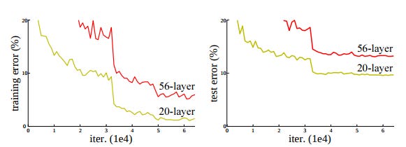
Fig: Training error (left) and test error (right) on CIFAR-10 with 20-layers and 50-layers 'plain' networks. The deeper network has higher training error, thus test error. (Img credit: https://arxiv.org/abs/1512.03385)
Researchers behind the ResNet architectures noticed that by increasing the depth of a plain network, training and test errors were actually worse than their shallow counterparts.
It is well known that increasing the depth leads to exploding or vanishing gradients problem if weights are not properly initialized. However, that can be countered by techniques like batch normalization.
In spite of that, deeper networks (like the 50-layer one in above image) experience degradation in convergence - with accuracy getting saturated and errors remaining higher than the shallower ones.
We needed a change of approach to counter challenges posed by deeper network.
Intuition behind Residual Networks
There are a couple of intuitions that we should understand before getting into the mechanics of ResNets.
Make it deep, but remain shallow
Given a shallower network - how can we take it, add extra layers and make it deeper - without losing accuracy or increasing error? It's tricky to do but one insight is that if the extra layers added to the deeper network are identity mappings, they become equivalent to the shallower network. And hence, they should produce no higher training error than it's shallower counterpart. This is called a solution by construction by the authors.

Fig: A Shallow network (left) and a deeper network (right) constructed by taking the layers of the shallow network and adding identity layers between them. Img Credit: (Img Credit: [Kaiming He])
Understanding residual
Let us revisit the mathematical concept of a Residual.
A residual is the error in a result.
Let's say, you are asked to predict the age of a person, just by looking at her. If her actual age is 20, and you predict 18, you are off by 2. 2 is our residual here. If you had predicted 21, you would have been off by -1, our residual in this case. In essence, residual is what you should have added to your prediction to match the actual.
What is important to understand here is that, if the residual is 0, we are not supposed to do anything to the prediction. We are to remain silent since the prediction already matched the actual.
This can be put into a nice little diagram.
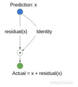
In the diagram, x is our prediction and we want it to be equal to the Actual. However, if is it off by a margin, our residual function residual() will kick in and produce the residual of the operation so as to correct our prediction to match the actual. If x == Actual, residual(x) will be 0. The Identity function just copies x.
The Residual Network
We can now weave the above two intuitions together to come to the logical conclusion of a ResNet.
So we want a deeper network where:
We want to go deeper without degradation in accuracy and error rate. We can do this via injecting identity mappings.
We want to be able to learn the residuals so that our predictions are close to the actuals.
That's what the Residual Network does. This is realized by feedforward neural network with shortcut connections. As the paper says:
Shortcut connections are those skipping one or more layers. In our case, the shortcut connections simply perform identity mapping, and their outputs are added to the outputs of the stacked layers. Identity shortcut connections add neither extra parameter nor computational complexity. The entire network can still be trained end-to-end by SGD with backpropagation, and can be easily implemented using common libraries without modifying the solvers.
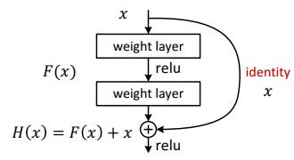
Fig: The reusable residual network. (Img credit:https://arxiv.org/abs/1512.03385)
The network can be mathematically depicted as:
H(x) = F(x) + x, where F(x) = W2*relu(W1*x+b1)+b2During training period, the residual network learns the weights of its layers such that if the identity mapping were optimal, all the weights get set to 0. In effect F(x) become 0, as in x gets directly mapped to H(x) and no corrections need to be made. Hence these become your identity mappings which help grow the network deep. And if there is a deviation from optimal identity mapping, weights and biases of F(x) are learned to adjust for it. Think of F(x) as learning how to adjust our predictions to match the actuals.
These networks are stacked together to arrive at a deep network architecture. For e.g., bellow is a ResNet arch with 34 layers.

Fig: A 34 layer ResNet with VGG 19 side by side (Img credit:https://arxiv.org/abs/1512.03385)
Similarly, researchers have stacked more layers as mentioned earlier, to increase the representational space which helped in gaining accuracy.
So that's that, our ResNet architecture!
What's next?
Kaiming He in one of his presentations does a comparison between ResNet and an Inception model (GoogLeNet), which is another state of the art architecture as of now. The Inception model, according to him, is characterized by 3 properties.
Bottleneck - reducing dimensions before applying expensive operations
Multiple Branches - extracting features of various sizes by using multiple and different filters parallelly
Shortcuts - as used in ResNet - to go deep
ResNet has two of the above properties, lacking multiple branches. That lead to the development of ResNeXt, which I will tackle in another post.
References